March Machine Learning Mania

Featured

Update: If you want more practice data projects, be sure to check out http://www.teamleada.com

In this post, we again use a third party data project taken from Kaggle, a company which hosts data science competitions. Since this was a competition for a prize and not in the interest of learning, users are no longer able to submit their predictions to Kaggle and receive a score. Therefore we thought we would just explain and post our process in participating in this competition. We hope this serves as another didactic example for people to follow along and since we are learners ourselves, we’d appreciate any feedback!

What You Will Learn:

These tutorials are meant for ANYONE interested in learning more about data analytics and is made so that you can follow along even with no prior experience in R. Some background in Statistics would be helpful (making the fancy words seem less fancy) but neither is it necessary. Specifically if you follow through each section of this tutorials series, you will gain experience in the following areas:

  • Implementing a machine learning model, namely Classification Trees
  • Creating custom functions in R
  • Constructing additional features to bolster your model
  • Using regular expressions
  • How to go from a data question/problem to a solution/prediction!

In Part I we will first breakdown the “March Machine Learning Mania” project and describe the steps to tackling this competition! It’s a little bit more challenging than the Titanic data project, and we’ll do our best to explain everything as concise as possible.

Why You Should Follow Along:

MIT Professor Erik Brynjolfsson likens the impact of Big Data to the invention of the microscope. Where the microscope enabled us to see things too small for the human eye, and what data analytics enables us to do now is see things previously too big. Just imagine the innovation that was spurred from the microscope. To believe in this parallel is to believe that we are coming upon an extremely exciting time!

Hal Varian, Chief Economist at Google, said this about the field of Data Analytics and Data Science:

If you are looking for a career where your services will be in high demand, you should find something where you provide a scarce, complementary service to something that is getting ubiquitous and cheap. So what’s getting ubiquitous and cheap? Data. And what is complementary to data? Analysis. So my recommendation is to take lots of courses about how to manipulate and analyze data: databases, machine learning, econometrics, statistics, visualization, and so on.

Who We Are:

We are recent UC Berkeley grads who studied Statistics (among other things) and realized two things: (1) how essential an understanding of Statistics and Data Analysis was to almost every industry and (2) how teachable these analytic practices could be!

Tips for Following Along

We recommend copying and pasting all code snippets that we have included. While copying and pasting allows you to run the code, you should read through and have an intuitive understanding of what is happening in the code. Our goal isn’t to necessarily teach R syntax, but to provide a sense of the process of digging into data and enable you to use other resources to better learn R.

New to R & RStudio?

No problem! But first go to our post to onboard you in Installing R, RStudio, and Setting Your Working Directory

Kaggle Project: March Machine Learning Mania

To have access to the data project, you also need to become a Kaggle Competitor. Don’t worry, it’s free! Sign up for Kaggle here. You can go directly to the March Madness Competition here. Please take a quick read of the competition summary, data, and evaluation. Unfortunately you cannot submit your model to Kaggle anymore. However they have posted the solutions and you can verify the accuracy of your model for yourself if you would like! We have also included all of the necessary data files here: DropBox With Kaggle Competition Data

The essence of this competition is quite simple. Most of us have probably filled out a bracket in March (whether we watched any of the regular season or not) and went on to ESPN to see which school Bill Simmons or Barack Obama thinks will make it to the Big Dance. Well now you can figure out for yourself whose going to win using data analytics! If you did this perfectly this season, Warren Buffett will given you a billion dollars!.

How to Begin

These competitions can be quite overwhelming, so it is good to break down the steps. In this part, we will go in-depth with each of the following steps:

  1. Taking a look at the datasets, noting column titles and rows
  2. Understanding the file you are submitting to Kaggle and more broadly what you are predicting
  3. Taking a step back now and brainstorming possible predictors!

Step One

Familiarizing Yourself with the Data

The first thing we need to do is download all of the datasets and load them into RStudio. You can download them all here or at this link here. Don’t forget to save them in a folder titled “Kaggle” in your desktop! If you’ve done one of our earlier tutorials, you’ve already made that very folder; the easier thing to do is to rename the existing folder (to say “Kaggle Titanic”) and recreate a new folder named “Kaggle” for the purpose of this tutorial. Also make sure you’ve correctly set up your working directory!

Inputting the Datasets in Rstudio

We again utilize the read.csv() function and set stringsAsFactors = FALSE which sets the columns of our data to be non-categorical and makes them easier to manipulate. Setting header = TRUE keeps the first rows as column titles instead of data.

For the code snippet below you may need to scroll left and right to copy and paste all of the code.

regSeason seasons teams tourneyRes tourneySeeds tourneySlots ```

We use ```head()``` and ```tail()``` functions to get an easy look at what these datasets contain. ```head()``` returns the first six rows and ```tail()``` returns the last six rows of the dataset. Specifically we will look at the two important ones, but you should check out all of them.

```R
head(regSeason)
tail(regSeason)

What do each of these columns represent? Read for more detail in the Kaggle descriptions. We also provide an easy dictionary below.

  • “season” = season organized alphabetically
  • “daynum” = Day Number of the season
  • “wteam” = Winning Team ID
  • “wscore” = Winning Team Score
  • “lteam” = Losing Team ID
  • “lscore” = Losing Team Score
  • “wloc” = Win Location (Home, Away, Neutral)
  • “numot” = Number of Overtimes (Not counted until season J)

Now lets take a look at the tournament results dataset.

head(tourneyRes)
tail(tourneyRes)

They are for the most part similar column names as those of the regSeason dataset.

Step Two

Understanding the End Goal

Understanding the submission file allows you to frame the dataset you need to create to build your model. At a high level, remember that we need to create two datasets which we will call Train and Test to build and utilize in our model. We’re using the Train to build the model, and make predictions based on Test data. Understanding what we are predicting enables you to understand the form of data as well as the data requirements for our model. Now, take a look at the “sample_submission.csv” file in the data provided by Kaggle.

In the first stage of the Kaggle competition, you must make predictions on every possible first-round tournament matchups between every team for seasons N, O, P, Q, and R (each alphabet represents a season). Taking season N as an example, there were a total of 65 teams, so you have to make predictions for Team 1 vs. Team 2, Team 1 vs. Team 3 …. Team 1 vs. Team 65 and then Team 2 vs. Team 3, Team 2 vs. Team 4, … Team 2 vs. Team 65 and so on until every combination is listed for each season N-R.

Below is a screenshot of the “sample_submissions.csv” file:
sample_sub

Notice how the format is SEASONLETTER_TEAMID_TEAMID for the “id” column. In the “pred” column, there will be numbers ranging from 0 to 1 representing the probability of the first TEAMID winning (the left side team).

“N_503_506” represents the season “N” and the first round matchup between team ID 503 vs. team ID 506. The “0” in the “pred” column represents the probability of team ID 503 winning (or alternatively team ID 506 losing).

Creating the Submission File

The code below is a little complicated and unnecessarily for understanding the project; it would probably be best to copy and paste now and interpret it later. What we create here is a custom function submissionFile() which creates columns in the form SEASONLETTER_TEAMID_TEAMID. We will explain how to create custom functions in more depth in our next post.

submissionFile playoffTeams numTeams matrix for(i in c(1:numTeams)) {
for(j in c(1:numTeams)) {
matrix[i,j] }
}
keep idcol for(i in c(1:numTeams)) {
for(j in c(1:numTeams)) {
if(keep[i,j] == T) {
idcol }
}
}
form return(form)
}
sub_file for(i in LETTERS[14:18]) {
sub_file }

Your First Submission!

The code below will create a file in your working directory (the Kaggle folder on your desktop) that you can submit to the competition! It’s always good to get a quick submission to get the ball rolling. Here we simply guess 50% for every possible matchup, which is the equivalent of flipping a fair-coin to predict each game! Obviously we can predict with better accuracy, especially for games such as a 1 Seed vs. a 16 Seed. That is to come later… But for now, we’ll make a random prediction to get a feel.

colnames(sub_file) sub_file$pred write.csv(sub_file, file = "sub1.csv", row.names = FALSE)

Step Three

Taking a Step Back, and Brainstorming!

This is the most creative part of data analytics and arguably the most important part. Now that you know what you are predicting, you want to think about how you want to predict it. These variables will be our predictors! Specifically how can we use the data Kaggle has given us to predict each matchup, and more broadly what are the indicators for any given team winning a game in March Madness? There is certain data that Kaggle doesn’t offer, that we may find intuitively significant or data we can create using the datasets Kaggle gives us.

  • Coaches Experience
  • Average Team Experience
  • Wins in the Last Six Games of the Season (We can create this!)
  • Shooting Percentage

The possibilities are only limited to your imaginations, especially given today’s technology in sensors and movement tracking! Its worth spending time brainstorming what indicators you think are important. Consult your basketball fanatic friends for tips. Now come back and see if you can recreate indicator variables based on what your friends advised you! We may even get to verify how truly “knowledgeable” your friends are about basketball!

Conclusion

You have successfully read in the data into RStudio and become more familiar with the data. You’ve also made your first submission! You might have a few possible variables you want to create to help with game outcome prediction. In Part II, we will work with the data and convert these variables into a data frame in RStudio. We’ll ultimately fit a machine learning model to make educated game outcome predictions! Thanks for reading!

In the mean time, checkout the Leaderboard page:
March Machine Learning Mania Leaderboard

Or go on to Part II here!

If you want more practice data projects, be sure to check out http://www.teamleada.com

Data Literacy in 2015

This will be a quick post.

It’s 2015 already. The word BigData and Data Science has been around for some time now, but it just doesn’t seem like enough people actually know what they’re talking about. That’s why we’re starting a movement called DataYear. The movement is meant to get people to work on data problems every other week. Leada is going to send you a new data set each week along with a few interesting data problems. Pledge to get your free updates! www.teamleada.com/data-year

jan1

StatsGuys

The Data Analytics Handbook: Researchers & Academics Edition

We just released our third and final edition of The Data Analytics Handbook! Interviewees include Hal Varian, the Chief Economist at Google and other academic professionals with deep expertise in the Big Data Industry.
Download and read it at http://www.analyticshandbook.com!

books-image

Here are the Top 5 Takeaways from our interviews!

TOP 5 TAKEAWAYS
FROM RESEARCHERS AND ACADEMICS

1. There are wrong questions to ask about data.
Included informally with Type I and Type II error in hypothesis testing should be Type III error. Type III error is asking the wrong questions about data or attempting to discern answers from data that actually isn’t available.

2. Data Science is a strategic initiative.
The huge demand for data scientists is a result of companies early investment in Big Data and wanting to get returns from those investments. As more companies invest in Big Data it will result in the strategic recruitment of more data scientists and data science departments.

3. Data professionals must be humble.
Not only are humble people better to work with, but a data literate professional must be humble to its data. He/she must be willing to accept when hypotheses are disproven and be skeptical of results. He/she must recognize that data is the main channel in which users communicate with a company now.

4. Analytics is a basis for competition.
The effective use of data is going to form the basis for competition for every industry in every organization.

5. For data science, learn how to learn.
We are still in the early stages of data science so the tools will constantly evolve, therefore education is a continuing process and should not be tied to any specific tool. As more tools get commercialized, the build, buy, or outsource decision firms must make is impossible to predict so to be competitive become adept at learning new tools.

The Data Analytics Handbook: CEOs & Managers Edition

Tags

Handbook_1_&_2We recently published our second edition of The Data Analytics Handbook which focuses on interviews with CEOs and Managers in the Data Science/Big Data Industry. We found the insight from these interviewees to be invaluable in understanding both the job market and the future of the Data Science industry. As a CEO you become a de-facto expert of your industry and many of these interviews showcase that expertise.

The list of interviewees is:

Mike Olson, CEO of Cloudera

Rohan Deuskar, CEO of Stylitics

Derek Steer, CEO of Mode Analytics

Greg Lamp, CTO of Y-Hat

Dean Abbott, CTO of Smarter Remarketer Inc.

Mary Gordon, Director of Analytics, Flurry

Dave Gerster, VP of Data Science, BigML

Tom Wheeler, Director of Education, Cloudera

Ali Syed, CEO of Persontyle

You can also checkout the website and download the handbook here: www.analyticshandbook.com

Be on the lookout for our third and final edition! The Data Analytics Handbook: Academia and Researchers edition with interviews from Hal Varian, Peter Norvig, and more!

March Machine Learning Mania Part III

Recap from Part II

In Part II we built our “Train” dataset. We used the predictors: Total win percentage, number of wins in the last six games, and seed in the tournament. Our response is the actual results of the NCAA tournament for the seasons A-M. In Part III we will build our machine learning model using classification trees. Using the “Train” dataset we “train our model”. Then we create our “Test” dataset and make predictions with our trained model.

Organization

  1. Applying a Classification Tree Model
  2. Creating our “Test” dataset
  3. Making Predictions using our Model
  4. Conclusion

Step One

Applying a Classification Tree Model

For a more in-depth explanation of how classification tree models work see this youtube video

R has a package called “Rpart” which allows us to apply the classification tree algorithm quite easily.

library('rpart')
train_rpart data =trainData, method = "class")

NOTE: There is an error with wordpress here you need to manually replace the ~ in the equation above for the Rcode to work.

Step Two

Creating our Test Data Set

The process for creating our “Test” data set is very similar to the process we did to create the “Train” data set. The difference is that whereas we used historical tournament results as our response, we now want to predict the match ups for all possible combinations of teams for tournaments N – R. Those match ups now define the teamIDs statistics we need to extract and we are now predicting the results using the model we built from the “Train” data.

We again have created a function that you can use to expedite this process. All you need to do is use a loop to create the “Test” data for each of the seasons.

testData for(i in LETTERS[14:18]) {
testData }

Step Three

Making Predictions

You should notice that our “Test” and “Train” datasets are in the exact same format with the exception of the “Win” column in the “Test” dataset being NA. We can again utilize a handy function in R predict() to make predictions using the model we built.

predictions_rpart predictions subfile write.csv(subfile, file = "model.csv", row.names = FALSE)

Step Four

Conclusion

Thanks for reading we hope it was informational! We would also appreciate any feedback from Kagglers on our process and variable selection! Other algorithms we implemented were SVM and GLM. We achieved the highest accuracy with Random Forests!

If you want more practice data projects, be sure to check out http://www.teamleada.com

The Data Analytics Handbook

Hello!

We are pleased to announce and release our latest resource on helping young professionals gain the skills and knowledge necessary to become data savvy in the 21st century!
data-analytics-cover

The Data Analytics Handbook is a compilation of interviews with Data Scientist and Data Analysts from some of the largest most dominant Big Data companies in the industry today. We hope you find our questions and their responses helpful, we know we learned a lot in the process of making this handbook!

Check out our page and download it right now here! Check it out!

And be on the lookout for our “CEOs and Managers” Edition! We specifically focus on how to attain a job in the Big Data Industry!

March Machine Learning Mania Part II

Recap

In Part I, we spent a lot of time familiarizing ourselves with the context of the project and the datasets that we are working with. Thoroughly doing this now can save hours of time later when you begin working with the data which we will now do in this post!

Part II Organization

  1. Introduction to Supervised Machine Learning
  2. Understanding the “Train” dataset we need to create to build our model
  3. Creating the “Train” dataset

Step One

Supervised Machine Learning

In trying to predict March Madness match ups from historical results we are engaging in a “Supervised Learning” task. This is a machine learning term which is used when you are inferring a function from training data. This function is then used to map predictions on new examples (our Test dataset).

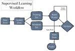
SupervisedWorkflow
This is an awesome chart of the workflow that is involved when you are doing a supervised machine learning task. A couple things to note.

  1. We scaled our data by taking the win percentage as a predictor rather than total wins or total losses. Scaling your data is important for accurate analysis.
  2. Validation set in the chart is the same as our “Test” dataset, specifically the most recent five seasons of the NCAA tournament not including the one going on right now!
  3. New data in the chart would be the regular season statistics for the current season thus allowing us to make March Madness predictions! Note we don’t do this here but you can go to Kaggle to see the data!
  4. We do this for fun so forget about the profit part 🙂

If you went through our first blog post on “Titanic: Machine Learning from Disaster” you would again see that using logistic regression is again an appropriate statistical model to make inferences from our “Train” dataset since what were predicting is win or lose is binary. From now on we will refer to what we are predicting as the response.

Step Two

Understanding the “Train” dataset

Lets go back and remember the variables you may have brainstormed which predict the match up of any given game. We will refer to these variables as the predictors which are used in our model to predict the response (win or lose). Some other variables we came up with that we will implement are:

  • Total Season Win Percentage
  • Number of Wins in A Teams Last 6 Games

Using Regular Season Statistics as Predictors

You should notice that our predictors are all team statistics for the regular season. Our assumption is that regular season performance is predictive of performance in the playoffs. So for any given playoff game we will use statistics from the regular season to predict the result. An added level of depth we must include is that we are predicting match ups which implies two teams. Therefore, we can use the regular season statistics from both teams to predict the result of the game. This data becomes our “Train” dataset to which we use to build our model.

Step Three

Creating the “Train” dataset

Since we have the regular season statistics and the playoff results for the past 18 seasons we can take a subset of this data and use it to “train a model”. The Kaggle competition directs us to what subset we should take, because they ask for predictions for the last 5 seasons we can use the first 15 as data to train our model. This process of taking a subset of the data to do analysis and then verifying your analysis with the remaining data is known as cross validation. To reduce variability this process is often done multiple times with different subsets of the data and then each result is averaged. Reducing variability is important because it indicates that our results are approximately similar to each other.

Determining our Response Values

We can use the results from each of the match ups in the 15 playoff tournaments as our response. In each of those games we know who played, their regular season statistics and who won. Therefore the first step is to create a data frame in R which lists these match ups in one column and the result of the game in another column.

Lets just try doing this with season A first. In the code below we first select the games from season A and name that data frame season_matches. Then we loop through each row of season_matches and we concatenate the season “A” with the teamID for the winning team and the losing team. We place these newly formed strings into a new data frame train_data_frame along with the result of the game.

season_matches <- tourneyRes[which(tourneyRes$season == "A"), ]
team <- vector()
result <- vector()
for(i in c(1:nrow(season_matches))) {
  row <- season_matches[i, ]
  if(row$wteam < row$lteam) {
    vector <- paste("A","_",row$wteam,"_", row$lteam, sep ="")
    team <- c(team, vector)
    result <- c(result, 1)
  } else {
    oth <- paste("A", "_", row$lteam, "_", row$wteam, sep ="")
    team <- c(team, oth)
    result <- c(result, 0)
  }
}
train_data_frame <- data.frame("Matchup" = team, "Win" = result)
head(train_data_frame)

Your console in RStudio should look something like this.
MatchupCol

Creating Your Predictors

Now that we have our response values we can begin to organize our predictors. To do this we first need to create a dataset which is organized by teamID rather than season. Again we will just do this for season A for brevity.

#Installing package
install.packages('stringr')
library('stringr')
#Selecting and sorting the playoff teamIDs least to greatest for season A
playoff_teams <- sort(tourneySeeds$team[which(tourneySeeds$season == "A")])

#Selecting the seeds for season A
playoff_seeds <- tourneySeeds[which(tourneySeeds$season == "A"), ]

#Selecting the regular season statistics for season A
season <- regSeason[which(regSeason$season == "A"), ]

#Wins by team
win_freq_table <- as.data.frame(table(season$wteam))
wins_by_team <- win_freq_table[win_freq_table$Var1 %in% playoff_teams, ]

#Losses by team
loss_freq_table <- as.data.frame(table(season$lteam))
loss_by_team <- loss_freq_table[loss_freq_table$Var1 %in% playoff_teams, ]

#Total Win Percentage
gamesplayed <- as.vector(wins_by_team$Freq + loss_by_team$Freq)
total_winpct <- round(wins_by_team$Freq / gamesplayed, digits = 3)
total_winpct_by_team <- as.data.frame(cbind(as.vector(loss_by_team$Var1), total_winpct))
colnames(total_winpct_by_team) <- c("Var1", "Freq")

#Num of wins in last 6 games
wins_last_six_games_by_team <- data.frame()
for(i in playoff_teams) {
  games <- season[which(season$wteam == i | season$lteam == i), ]
  numwins <- sum(tail(games$wteam) == i)
  put <- c(i, numwins)
  wins_last_six_games_by_team <- rbind(wins_last_six_games_by_team, put)
}
colnames(wins_last_six_games_by_team) <- c("Var1", "Freq")

#Seed in tournament
pattern <- "[A-Z]([0-9][0-9])"
team_seeds <- as.data.frame(str_match(playoff_seeds$seed, pattern))
seeds <- as.numeric(team_seeds$V2)
playoff_seeds$seed  <- seeds
seed_col <- vector()
for(i in playoff_teams) {
  val <- match(i, playoff_seeds$team)
  seed_col <- c(seed_col, playoff_seeds$seed[val])
}
team_seed <- data.frame("Var1" = playoff_teams, "Freq" =seed_col)

#Combining columns together
team_metrics <- data.frame()
team_metrics <- cbind(total_winpct_by_team, wins_last_six_games_by_team$Freq, team_seed$Freq)
colnames(team_metrics) <- c("TEAMID", "A_TWPCT","A_WST6", "A_SEED")

If you want to look at any of the data frame pieces we create, just utilize the head() function. For example:

head(wins_by_team)
head(team_metrics)

NOTE: For the actual competition we used the following predictors:

  • Away Wins Winning Percentage
  • Wins by margin less than 2
  • Losses by margin less than 2
  • Wins by margin greater than 7
  • Losses by margin greater than 7
  • Win Percentage in last 4 weeks
  • Win Percentage against playoff teams
  • Number of wins in last 6 games of the season
  • Seed in Tournament
  • Wins in Tournament

Putting the Pieces Together and Creating Your “Train” Dataset

So now we have our predictors organized by individual teams regular seasons statistics and we have our response which is the results of tournament play.

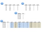
Take a look at the image below which shows the data frames we have created and how we want to combine them to create our “Train” dataset. Data frame (DF) 1 and DF 2 are the predictors organized by individual teams (team_metrics data frame), DF 2 is a copy of DF 1 with changed column names. You can also think of this as the home team and the away team data frames. DF 3 is the response, Win or Loss, and the teams that were involved in each of the games (train_data_frame). Remember, we only show the first six rows of each of these data frames!

Slide1

DF 4 is our “Train” data set. How did we get there? If you look the teamIDs on the left side for each of the “Matchups” in DF 3 you should notice that is the teamID order in which we need to re-order DF 1. Then if you look at only the teamIDs on the right side for the “Matchups” in DF 3 you should notice that that is the teamID order in which we need to re-order DF 2. Once you do so you have two new data frames organized in the correct order and when you bind the columns together you create the correct match ups and ultimately the “Train” data frame!

This is quite confusing so we will explain it step by step:
1. Sort DF 1 by the teamIDs defined in the column titled “A_ID” in DF 4
2. Sort DF 2 by the teamIDs defined in the column titled “B_ID” of DF 4
3. Combine the columns from the two data frames in 1 and 2 to create your “Train” data set!

We provide utility functions which do this process and over all seasons A-M. To use these functions and create your “Train” data set download the file “blog_utility.R” and place it in your “Kaggle” folder on your desktop, then use the following code. You can download the “blog_utility.R” file at this link.

source('blog_utility.R')
trainData <- data.frame()
for(i in LETTERS[1:13]) {
  trainData <- rbind(trainData, train_frame_model(i))
}

Take a look at the “Train” dataset we have just created with the head() function.

Conclusion

You have now created your “Train” data set with the the following predictors: Winning percentage, number of wins in the last six games of the season, and seed in the tournament! In the final post we will build our “Test” data set and build a machine learning model! Thanks!

You can go on to Part III here!

If you want more practice data projects, be sure to check out http://www.teamleada.com

Installing R, RStudio, and Setting Your Working Directory

Tags

Installing R and Rstudio

Here are step by step instructions for installing R and Rstudio. R is a useful and free application for data analytics that is widely used by statisticians and data miners. RStudio provides a more user friendly interface that will speed up your learning greatly!

Macs
Download and install R “3.0.3 pkg” here: Mac Install

Windows
Download and install R here: Windows Install

Linux
Download and install R here: Linux Install

Next, choose the appropriate package for RStudio here: RStudio Install

Setting Your Working Directory

Your working directory is the folder which you are directing R to extract and save files. First create a folder called “Leada” on your desktop.

Now in RStudio, we must create a file for us to write in. Go to File ==> New ==> Rscript. In this Rscript we must tell R where our current working directory is. We do this by using the setwd() function. Your working directory indicates to R which folder to look for the datasets you want to use. Remember everything in R you type is case sensitive!

For Mac Users:

getwd()

setwd("/Users/your_user_name/Desktop/Leada/")

If your confused you can use the image below as an example, the correct code would be:

setwd("/Users/Clair/Desktop/Leada/")

Path Image
For Windows users:

getwd()

setwd("C:/Users/your_user_name/Desktop/Leada")

Running you RCode

To run what you just wrote in your RScript, put your cursor on a line of code in your RScript and enter control and return at the same time! It should now pop up on the bottom left window labeled Console in blue, and if there is no red code that follows it has run correctly. Congrats you’ve just run your first line of R code! From now on you can run any of our code snippets by copy and pasting it into your own RScript, and entering control and return. Typingcontrol and return on any part of the line runs the entire line of RCode.

Happy Learning!

Data Analytics for Beginners: Part 2

Recap

In the last post, we prepared our working environment. We also got R/Rstudio working, loaded our data, and followed it up with a bit of visualization and exploration. Now that we have a better understanding of the data, we’re ready to move on to the next part: manipulating the data to prepare to plug it into a model.

Cleaning the TRAIN Data

After doing some exploratory analysis of the data, we now need to clean it to create our model. Note that it is important to explore the data so that you understand what elements need to be cleaned. For example you might have noticed that there are missing values in the data set, especially in the Age column.

Removing Variables Not Used for the Model

At this point, we remove the variables that we do not want to use in the training data for the model: PassengerID, Ticket, Fare, Cabin, and Embarked. To do so, we index our data set trainData with [ ]. The c() function generates a list of numbers. By including this list (along with a negative sign), we let R know to subset (or remove) those columns.

trainData = trainData[-c(1,9:12)]

Additionally, we need to replace qualitative variables (such as gender) into quantitative variables (0 for male, 1 for female etc) in order to fit our model. Note that there are models where the variables can be qualitative. We use the R function gsub() which will replace any text with a value of our choosing.

Replacing Gender variable (Male/Female) with a Dummy Variable (0/1)

Additionally, we need to replace qualitative variables (such as gender) into quantitative variables (0 for male, 1 for female etc) in order to fit our model. Note that there are models where the variables can be qualitative. We use the R function gsub() which will replace any text with a value of our choosing.

trainData$Sex = gsub("female", 1, trainData$Sex)
trainData$Sex = gsub("^male", 0, trainData$Sex)

Making Inferences on Missing Age Values

Lastly, upon examining our dataset, we see that many entries for “age” are missing. Because age entries could be an important variable we try inferencing them based on a relationship between title and age; we’re essentially assuming that Mrs.X will older than Ms.X. Moreover, we’re (naively) assuming that people with the same titles are closer together in age.

So first, we put the index of people with the specified surname into a list for further processing. In R we use the grep() function which will return a vector of row numbers which have a specified surname.

master_vector = grep("Master.",trainData$Name, fixed=TRUE)
miss_vector = grep("Miss.", trainData$Name, fixed=TRUE)
mrs_vector = grep("Mrs.", trainData$Name, fixed=TRUE)
mr_vector = grep("Mr.", trainData$Name, fixed=TRUE)
dr_vector = grep("Dr.", trainData$Name, fixed=TRUE)

You might have noticed that there are other less frequent titles such as Reverend or Colonel which we are ignoring for now.

Next, we rename each name with a shortened tag. This means replacing the full name of an individual, such as “Allison, Master. Hudson Trevor” we shorten it to be “Master”. This allows for a standardized column This is done in the following code:

for(i in master_vector) {
  trainData$Name[i] = "Master"
}
for(i in miss_vector) {
  trainData$Name[i] = "Miss"
}
for(i in mrs_vector) {
  trainData$Name[i] = "Mrs"
}
for(i in mr_vector) {
  trainData$Name[i] = "Mr"
}
for(i in dr_vector) {
  trainData$Name[i] = "Dr"
}

Note that we utilized a for loop, which we explain below.

FOR LOOP
For loop is intended to apply the same function, over a range of data.

Now that we have a series of standardized titles, we calculate the average age of each title.

Making Inference on Missing Age Values: Inputting Title-group averages

We replace the missing ages with their respective title-group average. This means that if we have a missing age entry for a man named Mr. Bond, we substitute his age for the average age for all passenger with the title Mr. Similarly for Master, Miss, Mrs, and Dr. We then write a for loop that goes through the entire Train data set and checks if the age value is missing. If it is, we assign it according to the surname of the observation. This code snippet is a bit complicated; you can just copy and paste for now if you’re not confident about understanding it!

master_age = round(mean(trainData$Age[trainData$Name == "Master"], na.rm = TRUE), digits = 2)
miss_age = round(mean(trainData$Age[trainData$Name == "Miss"], na.rm = TRUE), digits =2)
mrs_age = round(mean(trainData$Age[trainData$Name == "Mrs"], na.rm = TRUE), digits = 2)
mr_age = round(mean(trainData$Age[trainData$Name == "Mr"], na.rm = TRUE), digits = 2)
dr_age = round(mean(trainData$Age[trainData$Name == "Dr"], na.rm = TRUE), digits = 2)

for (i in 1:nrow(trainData)) {
  if (is.na(trainData[i,5])) {
    if (trainData$Name[i] == "Master") {
      trainData$Age[i] = master_age
    } else if (trainData$Name[i] == "Miss") {
      trainData$Age[i] = miss_age
    } else if (trainData$Name[i] == "Mrs") {
      trainData$Age[i] = mrs_age
    } else if (trainData$Name[i] == "Mr") {
      trainData$Age[i] = mr_age
    } else if (trainData$Name[i] == "Dr") {
      trainData$Age[i] = dr_age
    } else {
      print("Uncaught Title")
    }
  }
}

In the above code snippet, we use a if-statement. If statements are intended to help with decision making:

If-statement:
It executes a specific line of code, depending on certain true/false conditions.

if (some true/false statement_1) {
  #do this action if it is true
} else if (some other true/false statement_2) {
  #do this if the statement_1 wasn't true, but statement_2 ended up true
} else if (some other true/false statement_3) {
  #do this if the statement_1 and statement_2 were both not true, but statement_3 was true.
} else {
  #do this if none of the statement_* was true. Note that this last bit of "else" doesn't always have to happen.
}

Ultimately if statements allow people to let programs make decisions.

Quick Recap

At this point, we have accomplished the following:
– [x] load the data we intend to work with.
– [x] did some preliminary exploration into the data.
– [x] cleaned the data by converting the Sex variable to (0/1) and made inferences on the missing age entries.

Part of curating the data is also to create additional variables which we could use and may help with the classification and prediction of Test data passengers surviving.

Creating New Variables to Strengthen Our Model

By creating new variables we may be able to predict the survival of the passengers even more closely. This part of the walkthrough specifically includes three variables which we found to help our model. Think about what the added variables mean; do they make intuitive sense? How might these variables affect the survival rate?

Variable 1: Child.

This additional variable choice stems from the fact that we suspect that being a child might affect the survival rate of a passenger.

We start by creating a child variable. This is done by appending an empty column to the dataset, titled “Child”.
We then populate the column with value “1”, if the passenger is under the age of 12, and “2” otherwie.

trainData["Child"]
for (i in 1:nrow(trainData)) {
  if (trainData$Age[i] <= 12) {
    trainData$Child[i] = 1
  } else {
    trainData$Child[i] = 2
  }
}

Variable 2: Family

This variable is meant to represent the family size of each passenger by adding the number of Siblings/Spouses and Parents/Children (we add 1 so minimum becomes 1). We’re guessing that larger families are less likely to survive, or perhaps it is the other way around. The beautiful part is that it doesn’t matter! The model we build will optimize for the problem. All we’re indicating is that there might be a relationship between family size and survival rate.

trainData["Family"] = NA

for(i in 1:nrow(trainData)) {
  x = trainData$SibSp[i]
  y = trainData$Parch[i]
  trainData$Family[i] = x + y + 1
}

Varible 3: Mother

We add another variable indicating whether the passenger is a mother.
This is done by going through the passengers and checking to see if the title is Mrs and if the number of kids is greater than 0. This also includes any titles with Mrs and if the number of parents is greater than 0

trainData["Mother"] 
for(i in 1:nrow(trainData)) {
  if(trainData$Name[i] == "Mrs" & trainData$Parch[i] > 0) {
    trainData$Mother[i] = 1
  } else {
    trainData$Mother[i] = 2
  }
}

Now, we have a fully equipped training dataset!

Cleaning the TEST Data

Now that we have a cleaned and bolstered trainData, we repeat the exact process on the testData. The idea is to conduct the same steps (in terms of subsetting, cleaning, inference, adding more variables), so that both datasets are in the same state.

The only difference is the following: The test dataset doesn’t have the “Survived” variable (which is what we’re trying to predict), therefore the subsetting indexes are slightly different when cleaning the data. You should copy and paste the code below. Notice how similar the code is to what we used in trainData.

RCode to Clean the Test Data

PassengerId = testData[1]
testData = testData[-c(1, 8:11)]

testData$Sex = gsub("female", 1, testData$Sex)
testData$Sex = gsub("^male", 0, testData$Sex)

test_master_vector = grep("Master.",testData$Name)
test_miss_vector = grep("Miss.", testData$Name)
test_mrs_vector = grep("Mrs.", testData$Name)
test_mr_vector = grep("Mr.", testData$Name)
test_dr_vector = grep("Dr.", testData$Name)

for(i in test_master_vector) {
  testData[i, 2] = "Master"
}
for(i in test_miss_vector) {
  testData[i, 2] = "Miss"
}
for(i in test_mrs_vector) {
  testData[i, 2] = "Mrs"
}
for(i in test_mr_vector) {
  testData[i, 2] = "Mr"
}
for(i in test_dr_vector) {
  testData[i, 2] = "Dr"
}

test_master_age = round(mean(testData$Age[testData$Name == "Master"], na.rm = TRUE), digits = 2)
test_miss_age = round(mean(testData$Age[testData$Name == "Miss"], na.rm = TRUE), digits =2)
test_mrs_age = round(mean(testData$Age[testData$Name == "Mrs"], na.rm = TRUE), digits = 2)
test_mr_age = round(mean(testData$Age[testData$Name == "Mr"], na.rm = TRUE), digits = 2)
test_dr_age = round(mean(testData$Age[testData$Name == "Dr"], na.rm = TRUE), digits = 2)

for (i in 1:nrow(testData)) {
  if (is.na(testData[i,4])) {
    if (testData[i, 2] == "Master") {
      testData[i, 4] = test_master_age
    } else if (testData[i, 2] == "Miss") {
      testData[i, 4] = test_miss_age
    } else if (testData[i, 2] == "Mrs") {
      testData[i, 4] = test_mrs_age
    } else if (testData[i, 2] == "Mr") {
      testData[i, 4] = test_mr_age
    } else if (testData[i, 2] == "Dr") {
      testData[i, 4] = test_dr_age
    } else {
      print(paste("Uncaught title at: ", i, sep=""))
      print(paste("The title unrecognized was: ", testData[i,2], sep=""))
    }
  }
}

#We do a manual replacement here, because we weren't able to programmatically figure out the title.
#We figured out it was 89 because the above print statement should have warned us.
testData[89, 4] = test_miss_age

testData["Child"] = NA

for (i in 1:nrow(testData)) {
  if (testData[i, 4] <= 12) {
    testData[i, 7] = 1
  } else {
    testData[i, 7] = 1
  }
}

testData["Family"] = NA

for(i in 1:nrow(testData)) {
  testData[i, 8] = testData[i, 5] + testData[i, 6] + 1
}

testData["Mother"] = NA

for(i in 1:nrow(testData)) {
  if(testData[i, 2] == "Mrs" & testData[i, 6] > 0) {
    testData[i, 9] = 1
  } else {
    testData[i, 9] = 2
  }
}

Conclusion

At this point, we’ve finished preparing the data. testData and trainData will look very similar (after all they both underwent the very similar processes). Believe it or not, the hard part is over! Now that have clean Train and Test datasets, we will simply plug the Train data in a model (thus training the model). We then use the trained model to create predictions utilizing the Test data. The mathematically hardest part (solving some complex optimization problem within the model) is entirely done by R!

Go on to Part 3 Here

If you want more practice data projects, be sure to check out http://www.teamleada.com